
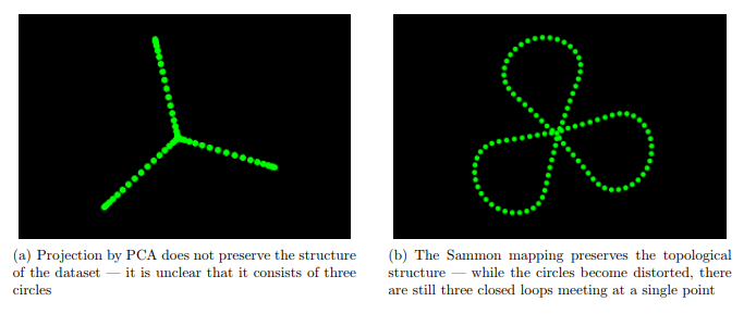
Sammon Mapping belongs to the multidimensional scaling algorithms family, as its main goal is to reduce a high dimensionality space to a lower dimensionality space, for visualization purposes. Unlike PCA and other dimensionality scaling algorithms, Sammon Mapping’s aim is not to highlight the most descriptive component to project the original data points onto, but rather to represent more or less the same “structure” of the original data, even when flattened in lower dimensionality space, highlighting patterns and spatial relationships.
Purpose
Drawing points in the space is pretty easy if the space is 1, 2 or 3 dimensional. In order to represent higher dimensional spaces, one could apply some dimensionality reduction algorithm, keeping the best 2 or 3 axes of the space, or some combination. This kind of projection usually distorts distances between points, mapping them in a space where they don’t have the same shape.
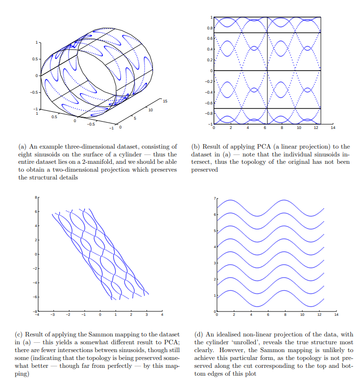
Sammon Mapping, instead, points to flatten a high dimensionality space preserving, when possible, the distance between any pair of points. It is a perfect startpoint for visualizing a high dimensionality dataset, searching for recurrent structures and shapes.
Images taken from here.
The algorithm
As proposed by J. W. Sammon in 1969 [1], Sammon Mapping is not actually an algorithm, strictly speaking. Sammon defined an error funcion, in order to evaluate how good a given projection is in preserving the original structure, by assessing the difference in the distance between each pair of points i and j in the higher and in the lower dimensionality space. Following his original proposal, the function error E is a function of the Euclidean distance, as follows:
where $ d_{ij}^{*} $ is the distance between i and j in the original space, and $ d_{ij} $ is the distance between i and j once mapped into the new, lower dimensionality space.
Thus, the projection itself is a optimization problem: for each pair of points {i, j}, we only need to find a new distance which is as close as possible to the original one, where “as close as possible” means beneath a given threshold $ \epsilon $. Sammon proposed a steepest gradient descent algorithm to minimize the error, a method easy to apply but poor in performances. In the following years several other approaches have been used, like simulated annealing [2] and neural networks [3].
Sun et al. [4] found out that using the left/right Bregman divergence as distance in the error function E is a major improvement for the whole algorithm in terms of performance.
By default, iterative algorithms for the Sammon error minimization problem don’t start from the original spatial configuration of datapoints, but from the Principal Component Analysis, as it has been shown to lead to a faster convergence.
The code
Unfortunately, it doesn’t look Python has a good library that includes the Sammon Mapping among its functions. The following code leverages a function taken from Tom Pollard’s repository. Thanks.
Here we go: we have a pandas dataframe listing some properties on 199 labelled seeds. Our dataset includes 7 features for each observation, making it impossible to draw…unless we reduce it to 3 or fewer dimensions with Sammon Mapping.
import pandas as pd
from sammon import sammon

df = pd.read_csv('../dataset/seeds.csv')

# sammon(...) wants a Matrix
X = df.as_matrix(columns = df.columns[:7])

# By default, sammon returns a 2-dim array and the error E
[y, E] = sammon(X)
Sammon Mapping in Python is simple as that, once you have your dataset the only thing to do is to convert it into a matrix, to feed sammon.py method with. The result is a n-dimensional array (where n=2 by default) you can plot.
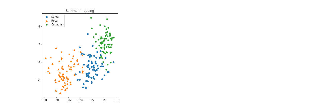
Why we can’t use the more popular Principal Component Analysis? Apparently there’s little difference:
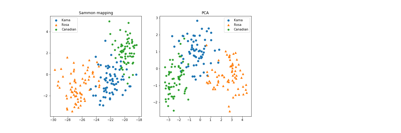
This time Sammon Mapping has found a projection very similar to the one PCA found. Maybe, by chance, the best way to preserve mutual distances between data points looks very close to the best way to magnify their variance. On the other hand, don’t forget that sammon starts from the PCA configuration for its iterations, and the default number of iterations (500) could be unsufficient to converge to some very different configuration with such a high dimensionality.
Let’s try with choosing 3 features to keep, as if our dataset was 3-dimensional.
import pandas as pd
from sammon import sammon

df = pd.read_csv('../dataset/seeds.csv')

# sammon(...) wants a Matrix
X = df.as_matrix(columns = ['Area', 'Perimeter', 'Compactness'])

# By default, sammon returns a 2-dim array and the error E
[y, E] = sammon(X)
As a reference, this plot shows the original spatial configuration of our datapoints, the result of Sammon Mapping and the Principal Component Analysis.
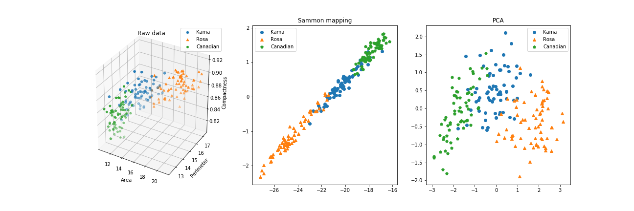
Here it is more clear: Sammon Mapping’s algorithm has found a way to represent the mutual distances between data points, while it doesn’t account for a better displacement on the screen. PCA, instead, found the two components that best capture the variance across the dataset, and draw it accordingly.
The full code of this demonstration is available at HERE.
Warning: Following Sammon’s definition, if the distance between two points i and j is 0, the algorithm will try a division by 0. Check for your data points to be non repeated, or your code will crash!
See also: PCA vs Sammon Mapping