Principal Component Analysis

Principal components analysis (PCA) is used when a simpler representation is desired for a set of intercorrelated variables. It is a method of transforming the original variables into new, uncorrelated variables. The new variables are called the principal components.

Purpose

This analysis occurs when the dataset includes many variables displaying strong pairwise correlations, its main purposes are:

reduce the number of variables from n to k where k < n,
avoid loss of relevant information contained in the data.

Each principal component is a linear combination of the original variables. One measure of the amount of information conveyed by each principal component is its variance. For this reason the reduction of dimensionality is attained by retaining, in statistical analysis, only the first components, i.e. those with larger variances, while the last components, i.e. the least informative (a variable with zero variance does not distinguish between the members of the population), are dropped.

Possible uses of PCA:

Regression modelling: reduce the number of predictors and rely on a selection of principal components. This helps avoiding problems of multicollinearity
Test normality of variables: if the principal components are not normally distributed, neither are the original variables
In segmentation problems where one wishes to cluster individuals according to some variables: if these are too many they can be replaced by principal components
As an exploratory tool that allows for a better understanding of the relationships among variables
PCA for Data Visualization when the dimension are greater then 3¹.

The algorithm

Suppose our sample is made by $\textbf{x}_{1}$ … $\textbf{x}_{m}$ indipendent drowing from some p-dimentional population with empirical mean shift to 0 and $\textbf{S}$ as sample covariance matrix. The algorithm starts searching for the first principal component for every observation $i$, that is it tries to determne the coefficients of the linear combination given by

$t_{1i}=a_{11}x_{1i}+a_{12}x_{2i}+\dots+a_{1n}x_{ni}$ where $i = 1 \dots m$

that maximize Var( $t_{1i}$ ) under the constraint $\textbf{a}_{1}'\textbf{a}_{1}=1$ .
Then it procedes searching for the second principal component, that is determining the coefficient of the linear combination given by

$t_{2i}=a_{21}x_{1i}+a_{22}x_{2i}+\dots+a_{2n}x_{ni}$ where $i = 1 \dots m$

that maximize Var( $t_{2i}$ ) under the constraint $\textbf{a}_{2}'\textbf{a}_{2}=1$ .
The algorith computes all the other k components. The final output is $t_{1i} \dots t_{ki}$ for every observation $i$ , such that Var( $t_{1i}$ )$>\dots>$Var($t_{ki}$). Since Var( $t_{1i}$ ) $= \textbf{a}_{2}'\textbf{S}\textbf{a}_{2}$ its maximum is the largest eigenvalue $\lambda_{1}$ , so $\textbf{a}_{1}$ is attained by choosing the correspective eigenvalue of $\textbf{S}$ .
The proportion of variance explained by the first $k$ components is given by $\frac{\lambda_{1}+ \dots + \lambda_{k}}{\lambda_{1}+ \dots + \lambda_{n}}$ .

A tricky part of using PCA in practice is to understand how many components are needed to describe the data.

You can determined $k$ by looking at the cumulative explained variance ratio as a function of the number of components. The k components you choose have to explain at least 70\% or 80\% of the variability of the data.
You can determined $k$ retaining the components whose eigenvalues $\lambda_{l}$ , with $l = 1 \dots k$ , are greater than the average $\sum_{j=1}^{n}\frac{\lambda_{j}}{n}$ .\

NOTE 1: Since the PCs are linear combinations of the original variables, if the assumption of normality is satisfied, they should look normal as well. It is often recommended to verify then that the first PCs are approximately normally distributed.
NOTE 2: The last PCs can help point out suspect observations.

Cons:

It is not possible to explain a very high proportion of the total variance with a small number of principal components. This could happen If the correlations among variables are all small, the dimensionality is close to p, the eigenvalues will be nearly equal and the PCs will duplicate the original variables.
Frequently in real-life situations, the interpretation of the components is not straightforward.

The code

import pandas as pd
from sklearn.decomposition import PCA
from sklearn.preprocessing import StandardScaler

# load dataset into Pandas DataFrame
df = pd.read_csv('../dataset/seeds.csv')

features = ['Area', 'Perimeter', 'Compactness', 'Kernel.Length', 'Kernel.Width', 'Asymmetry.Coeff', 'Kernel.Groove']
# Separating out the features
x = df.loc[:, features].values
# Separating out the target
y = df.loc[:,['Type']].values
# Standardizing the features
x = StandardScaler().fit_transform(x)

pca = PCA(n_components=2)
principalComponents = pca.fit_transform(x)
principalDf = pd.DataFrame(data = principalComponents
             , columns = ['principal component 1', 'principal component 2'])

pca_ex

Choosing the number of component

We will show the method 1.

pca = PCA().fit(df)
plt.plot(np.cumsum(pca.explained_variance_ratio_))
plt.xlabel('number of components')
plt.ylabel('cumulative explained variance')
plt.savefig('pca_ncomp.png', bbox_inches='tight')

pca_ncomp

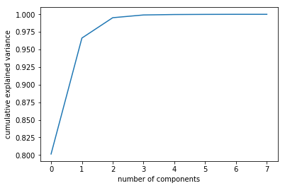
2 components seem to be a fair number.

Warning: PCA is affected by scale so you need to scale the features in your data. If you want to see the negative effect not scaling your data can have, scikit-learn has a section on the effects of not standardizing your data. HERE.

See also: PCA vs Sammon Sampling

1: Rencher A.C. and Christensen W.F. Methods of Multivariate Analysis, 3rd ed., Wiley, 2012